PINNs, Not the Spiky Kind.

Physics Informed Neural Networks (PINNs)

Physics-informed neural networks (PINNs) are a deep learning framework for solving partial differential equations (PDEs). PINNs work by adding a specified PDE to the loss function of a neural network and utilising automatic differentiation to train the network. This allows PINNs to solve PDEs that are difficult or impossible to solve with traditional numerical methods, such as finite element methods (FEM). Invented in 2017 by M. Raisse et al. in two papers ¹ for the forward/inverse problems, which are defined as follows:

• Foward Problem: The underlying equation and the boundary conditions are known, and the goal is to find the solution to the equation.
• Inverse Problem: The underlying equation and the boundary conditions are known, but the values of some of the parameters in the equation are unknown. The goal is to find the values of these parameters and the solution, given experimental data.

In both forward and inverse problems, PINNs are trained on a dataset of known solutions to the underlying equation. This dataset can be generated using numerical methods, such as the finite element method, finite difference method or from physical experiments. PINNs are particularly well-suited for solving problems where:

• The local consistency of FEM is broken like in integro-differential equations,
• High-dimensional input domain settings, in which classical techniques (such as FEM) are prohibitively expensive²,
• Parameter inference is occuring simultaneously (inverse problems).

Furthermore, they can be trained to generate solutions for multiple physical parameter values, by adding them as outputs from the model, e.g., multiple kinematic viscosity values in the Navier-Stokes equations. The PINN can also be probed for any continuous point in time/space unlike FEMs. In these restricted use cases, PINNs achieve performance on par or better than FEMs³. However PINNs are currently perform poorly at solving stiff equations, where stiffness is the difficulty to solve numerically, as 'Neural Networks are biased in their frequency domain to drop off lower frequency terms which is what causes the issues with stiffness' and in the vast majority of cases PDEs do not satisfy the conditions for which FEMs are considerably faster or more accurate. This means that in industry the most popular use case of PINNs is an out the box model that has been trained with standard boundary conditions, which allows the customer to get useful solutions out.

This article explores PINNs by generating a solution for the Sprott attractor (forward problem) and the solution to an inverse problem involving the Navier-Stokes equations. These problems are chosen to benefit a PINN as the Sprott attractor exhbits sensitivity to initial conditions which make it hard for the FEM to match. Furthermore inverse problems, as mentioned before, are faster for PINNs as they can learn the parameters while training unlike FEMs.

Deep Neural Networks

In PINNS, the neural network (NN) is approximating the solution to the PDE. The PDE is defined on the domain $\Omega \subset \mathbb{R}^d$ with a solution $u(\mathbf{x})$ approximated by the neural network $f$ parameterised by $\lambda$. The input vector is $\mathbf{x}=(x_{1},...,x_{d})^T$.

$$f \left( \mathbf{x};\frac{\partial u}{\partial x_{1}},...,\frac{\partial u}{\partial x_{d}};\frac{\partial^2 u}{\partial x_1^2},...,\frac{\partial^2 u}{\partial x_1\partial x_d},...;\lambda \right).$$

Alongside suitable boundary conditions $\mathcal{B}(u,\mathbf{x})=0 \text{ on } \delta \Omega$. Although many NN architectures exist, the multi-layer perceptron is suitable for solving most PDEs and as such for the remainder of the article the architecture will be assumed to be a fully connected feed-forward network.

Adapted Loss Function

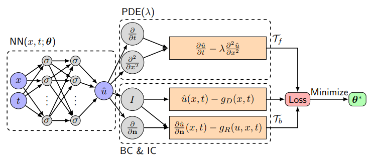
It was stated in the first paragraph that PINNs operate by $\textcolor{red}{\text{incorporating the PDE into the loss function}}$. So, in the usual manner, the model, loss and training dataset are denoted as $f$, $V$ and $\mathcal{T}$ respectively. Then $\mathbf{\theta}$ is defined as the weights and biases in the NN and $\mathcal{T}=\mathcal{T}_f \cup \mathcal{T}_b$ are two training sets where $\mathcal{T}_f \subset \Omega$ are the points in the domain and $\mathcal{T}_b \subset \Omega$ are the problem boundary conditions. Then the loss function can be setup as

$$\ell(\mathcal{T},f(x;\mathbf{\theta}),R) = \omega_f \textcolor{red}{R(f(\mathbf{x};\mathbf{\theta}),\mathcal{T}_f)} + \omega_b V(f(\mathbf{x};\mathbf{\theta}),\mathcal{T}_b)$$

where, for PINNs,

$$\textcolor{red}{R(f(\mathbf{x};\mathbf{\theta}),\mathcal{T}_f)}=\frac{1}{|\mathcal{T}_f|} \underset{x \in \mathcal{T}_f}{\sum} \left\lVert f(\mathbf{x};\frac{\partial u}{\partial x_{1}},...,\frac{\partial u}{\partial x_{d}};\frac{\partial^2 u}{\partial x_1^2},...,\frac{\partial^2 u}{\partial x_1\partial x_d},...;\lambda) \right\rVert_2^2$$ $$V(f(\mathbf{x};\mathbf{\theta}),\mathcal{T}_b)=\frac{1}{|\mathcal{T}_b|} \underset{x_i \in \mathcal{T}_b}{\sum} \lVert f(x_i;\mathbf{\theta}) - \mathcal{B}(x_i) \rVert_2^2$$

There are two terms for the loss, induced on the boundary conditions and on the domain, that are simultaneously backpropogated to train the model. Observed or experimental data can be added into the boundary condition loss set as $(x_i,\mathcal{B}(x_i))$ pairs. Building upon the classic misty hill analogy for gradient descent⁴, the $\textcolor{red}{R(f(\mathbf{x};\mathbf{\theta}),\mathcal{T}_f)}$ (the loss induced by the governing PDE) provides a set of steps down the hill that act as a good heuristic to improve the chances of getting to the bottom (global minima and solution to the PDE). For example if the aim is to approximate a solution to the diffusion equation $\frac{\partial^2 f}{\partial x^2}= \frac{1}{\kappa} \frac{\partial f}{\partial t}$ then the corresponding PDE loss would be $\underset{f}{\text{argmin}}\\,\left( \frac{\partial^2 f}{\partial x^2}- \frac{1}{\kappa} \frac{\partial f}{\partial t}\right)$ as the second expression is the minimisation task that corresponds to the NN obeying the PDE.

Automatic Differentiation

During the backpropogation process the traditional aim is to minimise the derivatives $\frac{\partial \ell(f)}{\partial x_1},...,\frac{\partial \ell(f) }{\partial x_d}$ ,i.e., the loss of the model with respect to the inputs. In the process of computing these derivatives we also end up computing the loss with respect to each model parameter and can then utilise a weight update algorithm such as ADAM⁵, L-BFGS⁶ or the traditional $w_{t+1}=w_t + \eta \frac{\partial \ell(f)}{\partial w}$. In PINNS we now have the boundary conditions of the PDE to enforce on the NN through the addition of the PDE error to the loss function. Furthermore, NNs only require one pass of the data through the approximating function however FEM require the computation of both $\\, f(x_1,...x_i,...,x_d)$ and $f(x_1,...x_i+ \Delta x_i,...,x_d)$ for all $i$. For large $\text{dim}(\mathbf{x})$, automatic differentiation is much more efficient.

The PINN

We now formalise the PINN algorithm and NN structure, copying from Lu Lu and DEEPXDE⁷.

1. Construct a Neural Network with accompanying parameters,

2. Create the two training datasets $\mathcal{T}_f,\mathcal{T}_b$,

3. Specify the loss function and weights associated to $\omega_f, \omega_b$,

4. Train the Neural Network to find find the best parameters that minimise the loss function.

   

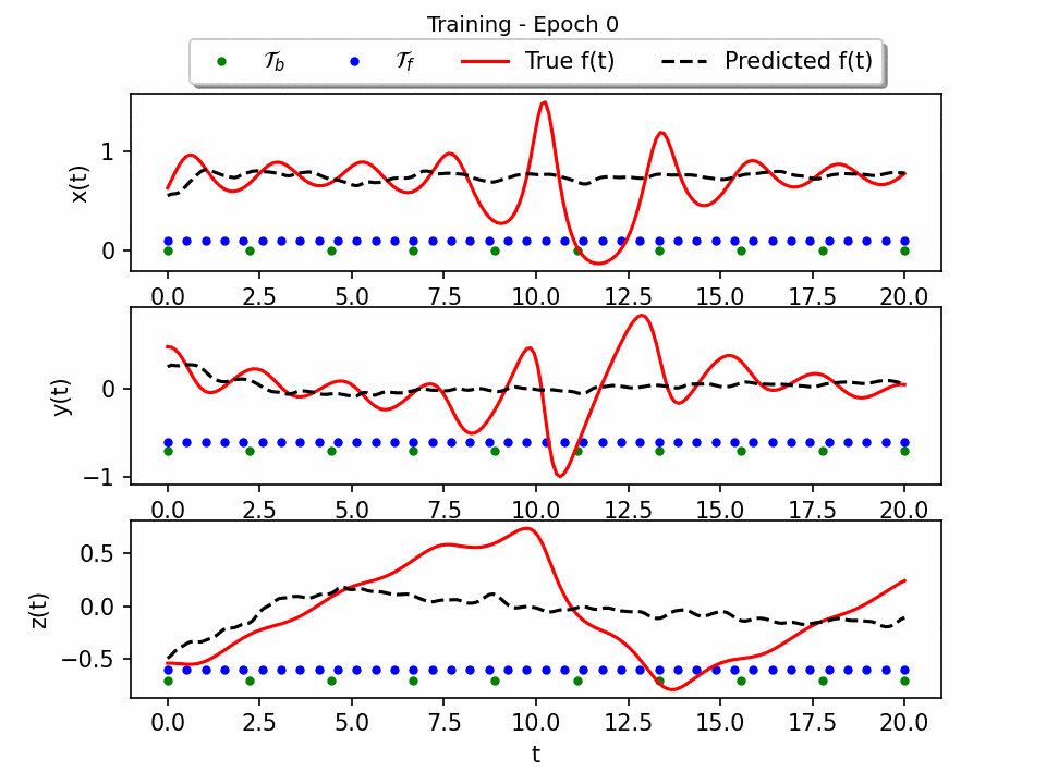
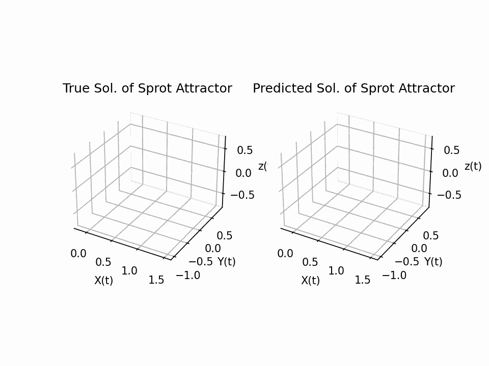
Forward Problem: Sprott Attractor

The Sprott Attractor⁸ is a chaotic dynamical system proposed in a 2014 paper that exhibits sensitivity to initial conditions and exhibits complex structure. It will be treated as a forward problem and therefore that we know in advance the parameters $\alpha, \beta$ and select $t \in [0,20]$ as the domain to learn on.

$$f(t)=\begin{cases} \frac{dx}{dt} = y +\alpha xy + xz \\ \frac{dy}{dt} = 1 - \beta x^2 + yz \\ \frac{dz}{dt} = x - x^2 - y^2 \end{cases},\quad \alpha=2.07, \beta = 1.79$$

Data/PDE Setup

The code in this section defines the geometric domain(time domain $(0,20)$), solver settings, and ODE system. The ODE system is a three-dimensional system of ordinary differential equations (ODEs) where $\texttt{x, y and z}$ are the three state variables of the system and $\texttt{o}$ is now the output of the model.

import deepxde as dde
import numpy as np

geom = dde.geometry.TimeDomain(0, 20)
dde.config.set_default_float("float64")
a = 2.07
b = 1.79


def ode_system(t, o):
    # https://www.dynamicmath.xyz/strange-attractors/ Sprott attractor

    x = o[:, 0:1]
    y = o[:, 1:2]
    z = o[:, 2:3]
    dx_t = dde.grad.jacobian(o, t, i=0)
    dy_t = dde.grad.jacobian(o, t, i=1)
    dz_t = dde.grad.jacobian(o, t, i=2)
    return [
        dx_t - (y + (x * a * y) + (x * z)),
        dy_t - 1 + b * x * x - y * z,
        dz_t - X + x * x + y * y,
    ]

Neural Network Setup

The code in this section sets up the neural network for solving the ODE system. The network architecture is 4 hidden layers, each with 20 neurons. The activation function for all layers is $tanh$ (notable for PINNS due its non-zero derivatives mitigating the "dying ReLU" problem⁹). The weights of the neural network are initialized using the Glorot normal initializer.

The code also defines a function called input_transform. This function takes a time $\texttt{t}$ as input and returns a vector of sinusoidal features that will be used as input to the neural network. As we know in advance that the solution contains sinusoidal like behaviour this feature layer will boost learning performance. The code then calls the \texttt{apply_feature_transform} method on the neural network.

The code in this section is used to set up the neural network for solving the ODE system.

n = 10
x_true, y_true, z_true = gen_truedata(n)

t = np.linspace(0, 20, n).reshape(n, 1)
observe_x = dde.icbc.PointSetBC(t, x_true, component=0)
observe_y = dde.icbc.PointSetBC(t, y_true, component=1)
observe_z = dde.icbc.PointSetBC(t, z_true, component=2)
data = dde.data.PDE(geom,ode_system,[observe_x,observe_y,observe_z],40,10,anchors=t,num_test=100)
layer_size = [1] + [20] *4 + [3]
activation = "tanh"
initializer = "Glorot normal"
net = dde.nn.FNN(layer_size, activation, initializer)

def input_transform(t):
    return tf.concat(
        (
            t,
            tf.sin(t),
            tf.sin(2 * t),
            tf.sin(3 * t),
            tf.sin(4 * t),
            tf.sin(5 * t),
            tf.sin(6 * t),
        ),
        axis=1,
    )


net.apply_feature_transform(input_transform)

Train

The code in this section trains the neural network to solve the ODE system. The training process uses the Adam optimizer with a learning rate of 1e-3. The training is run for 200 iterations, and the loss history is monitored every iteration. The model is saved to a file after training is complete for later inference.

model = dde.Model(data, net)
model.compile("adam", lr=1e-3,)
losshistory, train_state =model.train(iterations=200,
                                    display_every=1,
                                    disregard_previous_best=False, ) 
model.save(save_path="/strange_attract-10t/model")

Results

The results show that the Sprott Attractor model can be accurately solved using a neural network with only 50 pieces of data. The model converges after 80 epochs, and the final plot of the three-dimensional attractor matches the true solution with a testing error of approximately 1e-4. This is a significant result, as it shows that PINNS can be used to solve complex ODE systems with relatively little data. The attractor is a three-dimensional object that has a complex and unpredictable structure. The neural network is able to reproduce this structure accurately.

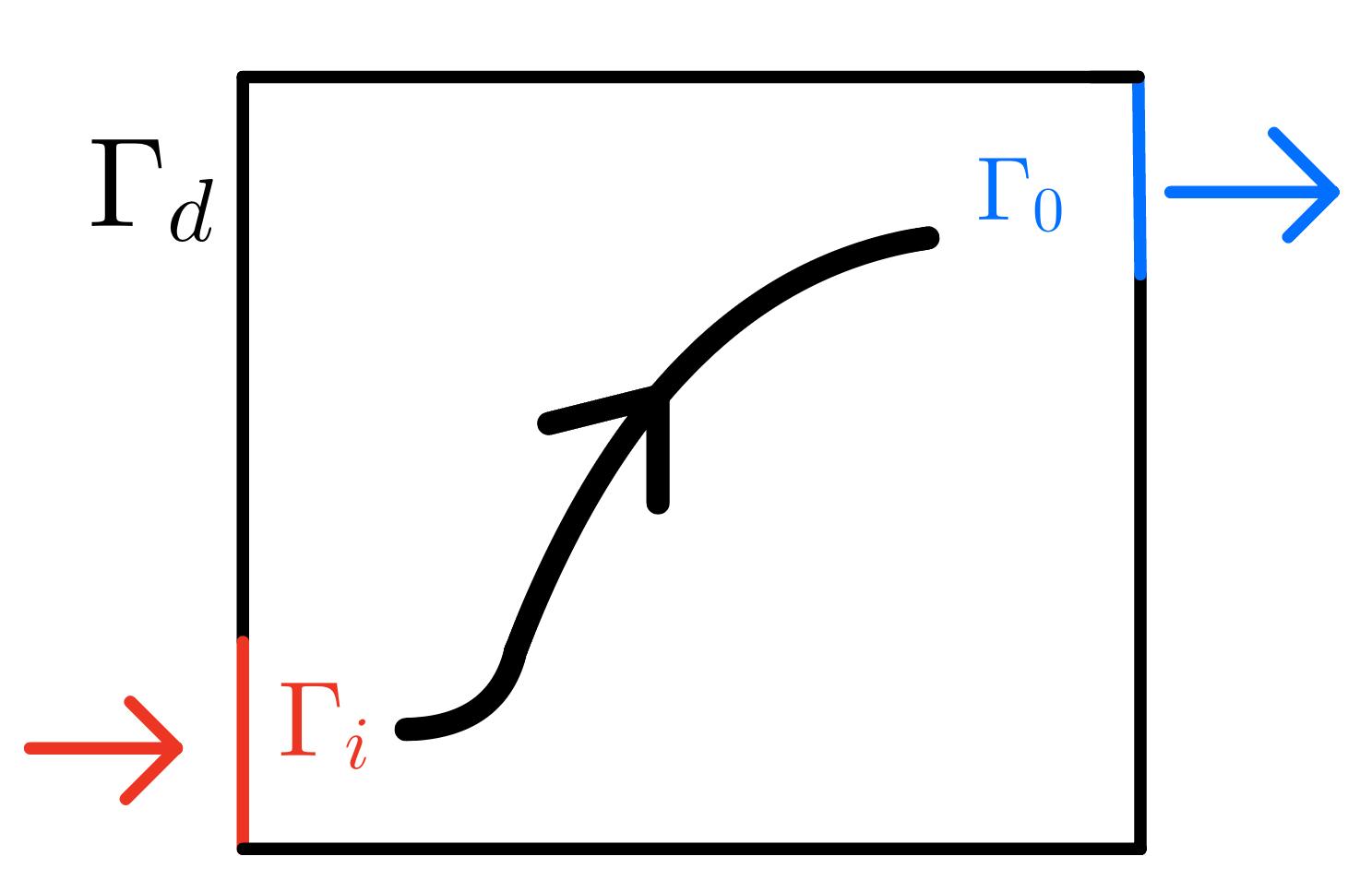
Inverse Problem: Inlet/Outlet Cavity

For the inverse problem, we consider a cavity filled with liquid that has an inlet port in the bottom left and outlet port in the top right, we aim to model the flow of liquid in this cavity.

The problem considered is one created by John Burkardt in 'Centroidal voronoi tesselation-based reduced-order modelling of complex systems'¹⁰ as the problem considered has an accompanying dataset¹¹ of $(u,v)$ pairs for the domain that can be used for $\mathcal{T}_b$. The spatial domain is defined as $\Omega = (0,1)\times(0,1)$, time domain $(0,T)$ and use the 2d Navier-Stokes Equations with the following boundary conditions:

$$\begin{align} \frac{\partial \mathbf{u}}{\partial t} - \nu \Delta \mathbf{u} + \mathbf{u} \cdot \nabla \mathbf{u} + \nabla p = 0 \quad \text{in} \quad (0,T)\times\Omega \\\ \nabla \cdot \mathbf{u} = 0 \quad \text{in} \quad (0,T)\times\Omega \\\ \mathbf{u}(0,x)=\mathbf{u}_0(x) \quad \text{in} \quad \Omega \\\ \\\ \mathbf{u}=5(1-(y-0.1)^2/0.01) \quad \text{on} \quad (0,T)\times\Gamma_i \\\ (\mathbf{n}\cdot\nabla)\mathbf{u}=0 \quad \text{on} \quad (0,T)\times\Gamma_o \\\ \mathbf{u}=0\quad \text{on} \quad (0,T)\times\Gamma_d \end{align}$$

Data/PDE Setup

The code in this section defines the Navier-Stokes equations that will be solved. The equations are defined in terms of the velocity field $(u,v)$, the pressure $p$, and the streamfunction $\psi$.We make the assumption that $u = \psi_y \text{ and } v = −\psi_ x$ for some latent function $\psi(t, x, y)$. Under this assumption, the continuity equation $u_x +v_y=0$ will be automatically satisfied.

The free parameters $[C_1,C_2]$ to be learned, that make the problem inverse, are also defined. The code then defines the spatial and temporal domains for the problem. The spatial domain is a rectangle with dimensions $(0,0) \text{ to } (1,1)$. The temporal domain is the interval [0,6]. The geometry is a combination of the spatial and temporal domains. In the code below we manufacture adherance to the continuity equation $\nabla \cdot \mathbf{u}=0$ by using the stream function¹² $\psi(x,y)$ which only needs continuous first and second partial derivatives (implying the order of differentiation does not matter) and obeys $u(x,y)=\frac{\partial \psi}{\partial y}\\, \text{ and }\\,v(x,y)=-\frac{\partial \psi}{\partial x}$. Then, the continuity condition holds as follows:

$$\nabla (u,v) \equiv \frac{\partial u}{\partial x} + \frac{\partial v}{\partial y} = \frac{\partial \psi}{\partial y \partial x} - \frac{\partial \psi}{\partial x \partial y} = 0.$$

So the model has four outputs $(\psi,p,u,v)$ where $u,v$ are linked to $\psi$ with the PDE equations u_diff = u_real - u and v_diff = v_real - v. This allows the point set boundary condition to be applied in the next section.

import deepxde as dde
import numpy as np
from create_datasets import create_dataset
# Parameters to be identified
C1 = dde.Variable(0.8)
C2 = dde.Variable(1 / 300)

def Navier_Stokes_Equation(x, y):
    """
        System of PDEs to be minimized: incompressible Navier-Stokes equation in the
        continuum-mechanics based setup.

        """
    psi, p, u_real, v_real = y[:, 0:1], y[:, 1:2], y[:, 2:3], y[:, 3:4]

    p_x = dde.grad.jacobian(p, x, i=0,j=0)
    p_y = dde.grad.jacobian(p, x, i=0,j=1)

    u = dde.grad.jacobian(psi, x, i=0, j=1)
    v = - dde.grad.jacobian(psi, x, i=0, j=0)

    u_x = dde.grad.jacobian(u, x, i=0, j=0)
    u_y = dde.grad.jacobian(u, x, i=0, j=1)
    u_t = dde.grad.jacobian(u, x, i=0, j=2)

    v_x = dde.grad.jacobian(v, x, i=0, j=0)
    v_y = dde.grad.jacobian(v, x, i=0, j=1)
    v_t = dde.grad.jacobian(v, x, i=0, j=2)

    du_xx = dde.grad.hessian(u, x, i=0, j=0)
    du_yy = dde.grad.hessian(u, x, i=1, j=1)
    dv_xx = dde.grad.hessian(v, x, i=0, j=0)
    dv_yy = dde.grad.hessian(v, x, i=1, j=1)

    continuity = u_x + v_y
    x_momentum = u_t + C1 * (u * u_x + v * u_y) + p_x - C2 * (du_xx + du_yy)
    y_momentum = v_t + C1 * (u * v_x + v * v_y) + p_y - C2 * (dv_xx + dv_yy)
    u_diff = u_real - u
    v_diff = v_real - v
    return continuity, x_momentum, y_momentum, u_diff, v_diff

space_domain = dde.geometry.Rectangle([0, 0], [1, 1])
time_domain = dde.geometry.TimeDomain(0, 6)
geomtime = dde.geometry.GeometryXTime(space_domain, time_domain)

Neural Network Setup

The code in this section sets up the neural network for solving the Navier-Stokes equations. The neural architecture has 6 hidden layers, each with 50 neurons. As before, the activation function for all layers is $tanh$ and the weights of the neural network are initialized using the Glorot uniform initializer.

The code also creates a dataset of training data. The dataset is created by sampling the Navier-Stokes equations on a fine grid. The dataset includes 700 domain points, 200 boundary points, 100 initial points for $\mathcal{T}_f$ and 7000 for $\mathcal{T}_b$, and 3000 test points.

[ob_x, ob_y, ob_t, ob_u, ob_v] = create_dataset('data_full.csv',5000)
ob_xyt = np.hstack((ob_x, ob_y, ob_t))
observe_u = dde.icbc.PointSetBC(ob_xyt, ob_u, component=2)
observe_v = dde.icbc.PointSetBC(ob_xyt, ob_v, component=3)

data = dde.data.TimePDE(
    geomtime,
    Navier_Stokes_Equation,
    [observe_u, observe_v],
    num_domain=700,
    num_boundary=200,
    num_initial=100,
    anchors=ob_xyt,
    num_test=3000
)

layer_size = [3] + [50] * 6 + [4]
activation = "tanh"
initializer = "Glorot uniform"
net = dde.nn.FNN(layer_size, activation, initializer)
model = dde.Model(data, net)

Train

The code in this section trains the neural network to solve the ODE system. The training process uses the Adam optimizer with a learning rate of 1e-3. The training is run for 10000 iterations and the loss history is monitored every 10 iterations. The model is saved to a file after training is complete for later inference.

This model required hours of time to train with a GPU accelerated tensorflow backend, so we highly recommend doing the same if you try to replicate the experiment.

model.compile("adam", lr=1e-3, external_trainable_variables=[C1, C2])
loss_history, train_state = model.train(
    iterations=10000, callbacks=[variable], display_every=10,
                     disregard_previous_best=False,)
model.save(save_path="/psi_pinn_nt/model")

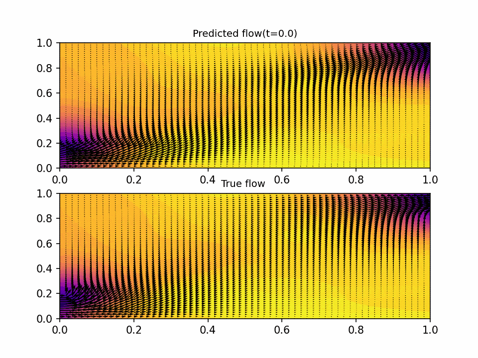
Results

The results show that the PINN is able to accurately predict the flow of fluid in the domain. The predicted flow matches the true flow over the domain the NN was trained on, with non-degenerative performance on out of domain data. The testing error was on the order of 1e-3 across the six objective functions, which is a good indication that the neural network is accurately predicting the flow.

Conclusion

I learned a lot about PINNs in the process of writing this article, specifically, testing my patience after spending one week debugging the PINN to discover that my visualization function was malformed. I learned about the basic structure of a PINN, how they are trained, and how they can be used to solve PDEs. I also learned about the advantages of PINNs over traditional numerical methods, such as FEM. I am excited to learn more about PINNs and their potential applications in the future.

Here are some specific things I learned:

• PINNs are a relatively new research area, but they have already shown great promise for solving PDEs.
• PINNs can be used to solve PDEs that are difficult or impossible to solve with traditional numerical methods.
• PINNs can be trained on relatively little data, how little data was required to train the Sprott attractor was very impressive.
• PINNs can often be more efficient than traditional numerical methods for high dimensional problems.

Thank you to Cam, Nathan, Rick and Ed for their support and putting up with my whining at spending one week debugging a single line of code and to Ben and James for their exhaustive grammar checking.

Footnotes

1. M. Raissi, P. Perdikaris, G.E. Karniadakis, Physics-informed neural networks: A deep learning framework for solving forward and inverse problems involving nonlinear partial differential equations ↩

2. Christian Beck et al, Overcoming the curse of dimensionality in the numerical approximation of Allen–Cahn partial differential equations via truncated full-history recursive multilevel Picard approximations ↩

3. Physics-Informed Neural Networks (PINNs) - Chris Rackauckas | Podcast #42 ↩

4. What can we learn from gradient descent? ↩

5. Kingma, D. P., & Ba, J. L. (2015). Adam: A method for stochastic optimization. ↩

6. Liu, D. C., & Nocedal, J. (1989). On the limited memory BFGS method for large scale optimization. ↩

7. LU LU, XUHUI MENG, ZHIPING MAO, AND GEORGE EM KARNIADAKIS, DEEPXDE: A DEEP LEARNING LIBRARY FOR SOLVING DIFFERENTIAL EQUATIONS ↩

8. J.C. Sprott, A dynamical system with a strange attractor and invariant tori ↩

9. Kenneth Leung,The Dying ReLU Problem, Clearly Explained ↩

10. JOHN BURKARDT, MAX GUNZBURGER, AND HYUNG-CHUN LEE, CENTROIDAL VORONOI TESSELLATION-BASEDREDUCED-ORDER MODELING OF COMPLEX SYSTEMS ↩

11. INOUT_FLOW2 INOUT Flow Problem Solution Datasets ↩

12. JOHN BURKARDT, The Stream Function, MATH1091: ODE methods for a reaction diffusion equation ↩