Project overview
This article covers the design of an agent-based Bitcoin market (BTC/GBP) inside a limit order book (LOB) and test whether it reproduces core stylised facts — heavy-tailed returns, volatility clustering, and a unit-root price process. The market mixes rule-based chartists with noise traders, extends Cocco et al.’s specification (Cocco et al., 2019), and benchmarks the output against real BTC data.
Agent architecture
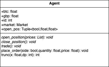
All agents inherit from an abstract base class that holds cash and crypto balances, a handle to the market, and helpers for opening or closing positions.
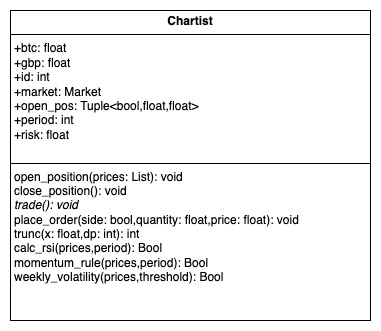
Chartists
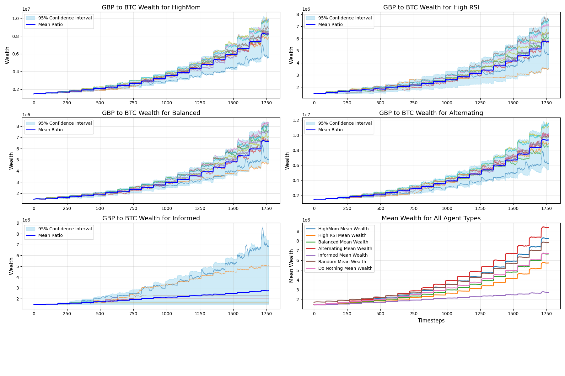
Chartists follow technical rules driven by either momentum or RSI signals, mirroring the setup analysed by Cocco, Tonelli, and Marchesi. Four subtypes alter the weighting between the rules:
| Subtype | Weighting |
|---|---|
| HighMom | 0.8 |
| HighRSI | 0.2 |
| Balanced | 0.5 |
| Alternating | "alt" |
For non-alternating subtypes, a uniform random draw chooses the strategy:
Alternating chartists inspect the weekly volatility of the last 30 prices:
def weekly_volatility(self, prices, threshold=0.025):
    if len(prices) < 30:
        return False
    recent_daily_returns = pd.DataFrame(prices[-30:])
    daily_std_dev = recent_daily_returns.pct_change(1).std()[0]
    weekly_volatility = daily_std_dev * np.sqrt(7)
    return weekly_volatility > threshold
An excerpt of the order placement logic highlights how RSI and momentum signals translate into limit orders:
if self.open_pos is None and mom:
    action = 1  # Buy
    delta = (prices[-1] - prices[0]) / len(prices)
    period = random.randint(1, len(prices) // 2)
    price = prices[-1] + 0.9 * (delta * period)
    quantity = self.risk * curr[action] / price
    self.place_order(action, trunc(quantity), price)
Noise traders
Noise traders inject stochastic liquidity, capturing the volatility effects highlighted in recent agent-based market studies (Dai et al., 2023). At each step they either open or close a position at a randomly sampled price:
The expected transaction amount is therefore
producing net-neutral pressure in expectation while amplifying return variance.
| Aspect | Random Traders | Chartists |
|---|---|---|
| Decision process | Uniform random choices | Technical indicators (RSI, momentum) |
| Motivation | Liquidity/noise | Profit-seeking |
| Price targeting | Normal around current price | Directional based on indicator |
| Market impact | Adds noise, occasionally dampens trends | Reinforces prevailing trends |
| Risk management | None | Agent-specific appetite (self.risk) |
Market design
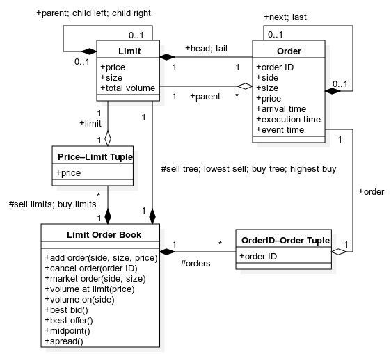
The market wraps Kautenja’s LOB implementation, enabling partial order fills and price-time matching. Three key adaptations were required to satisfy cryptocurrency constraints:
- Fractional Bitcoin: Orders can trade BTC to 5 decimal places, matching exchange minimums (e.g., Kraken Support).
- Position flexibility: Agents may submit any sequence of buys and sells subject to available balances—no enforced “flat” state.
- Fractional price response: The price impact function drops the floor operator so the tick size is continuous (Petrov, 2019).
r_n(ΔN_n) = α · sgn(ΔN_n) · √(|ΔN_n|).
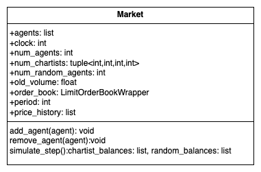
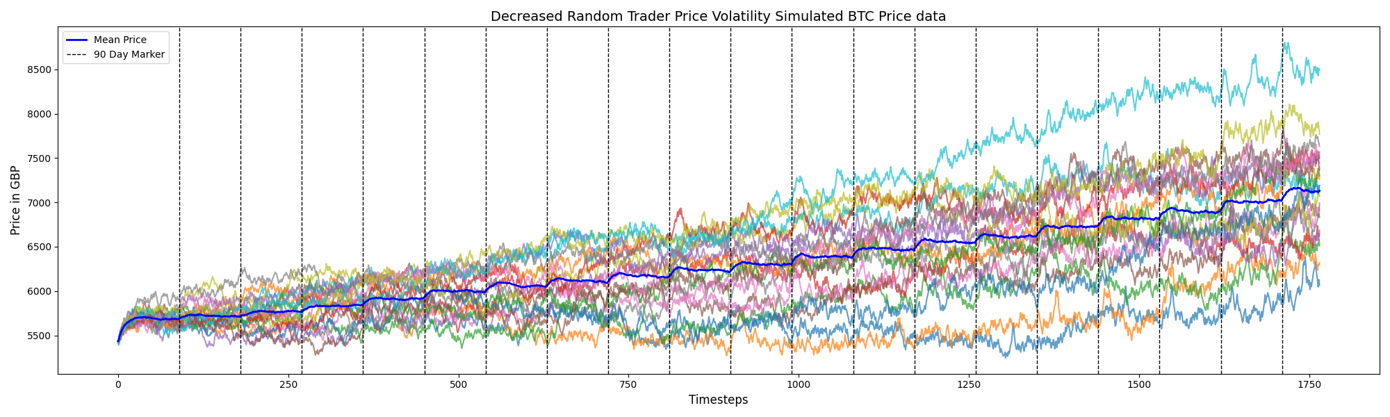
The simulate_step routine shuffles agents each turn, lets them trade, applies the price impact rule, and appends the updated price to history. Wealth injections of 10% emulate capital inflows observed in crypto markets and help trigger momentum. Baseline supply, address counts, and price levels follow January 1st 2020 observations of the BTC network (BitInfoCharts; Blockchain.com; Yahoo Finance).
Stylised facts reproduced
The model replicates Cocco et al.’s findings that, in a chartist/noise-trader ecosystem, returns remain heavy-tailed and volatility clusters even without fundamental value traders (Cocco et al., 2019).


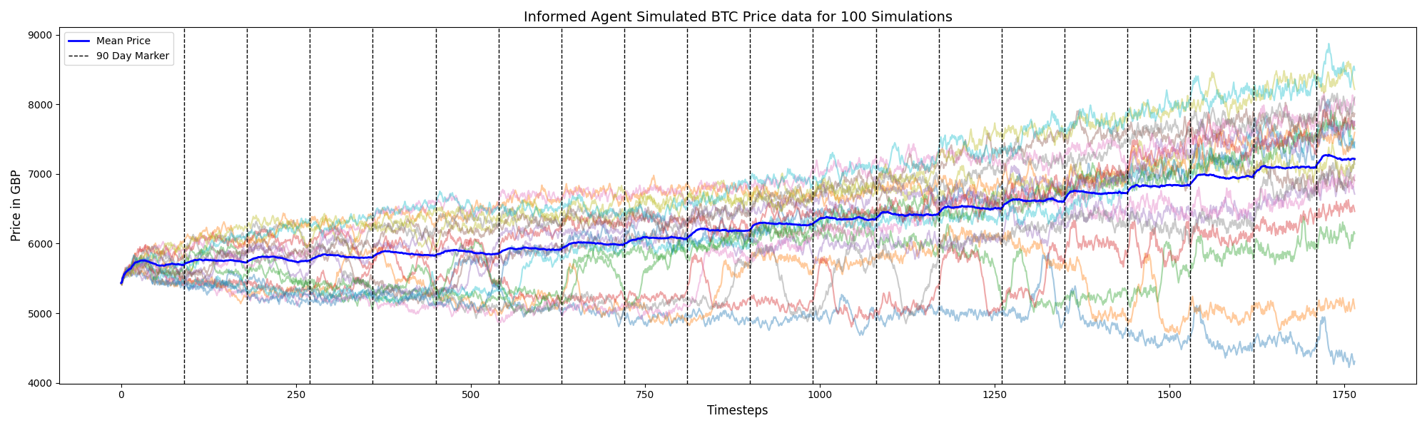
Activating informed momentum (RSI + alternating chartists) and periodic wealth injections magnifies these effects without breaking plausibility.

Momentum lookback windows ( n \in [1, 30] ) balance the Efficient Market Hypothesis—which argues that historical prices offer little predictive power (Fama, 1970)—with empirical evidence of short-lived inefficiencies in equity and cryptocurrency markets (Jiang, 2011; Al-Yahyaee et al., 2020). The shorter horizons allow chartists to exploit transient order-imbalance and liquidity effects without contradicting longer-run market efficiency.
Comparison with Cocco et al.
Price trajectories, volume, and mean reversion were benchmarked against Section 3 of the reference model (Cocco et al., 2019).
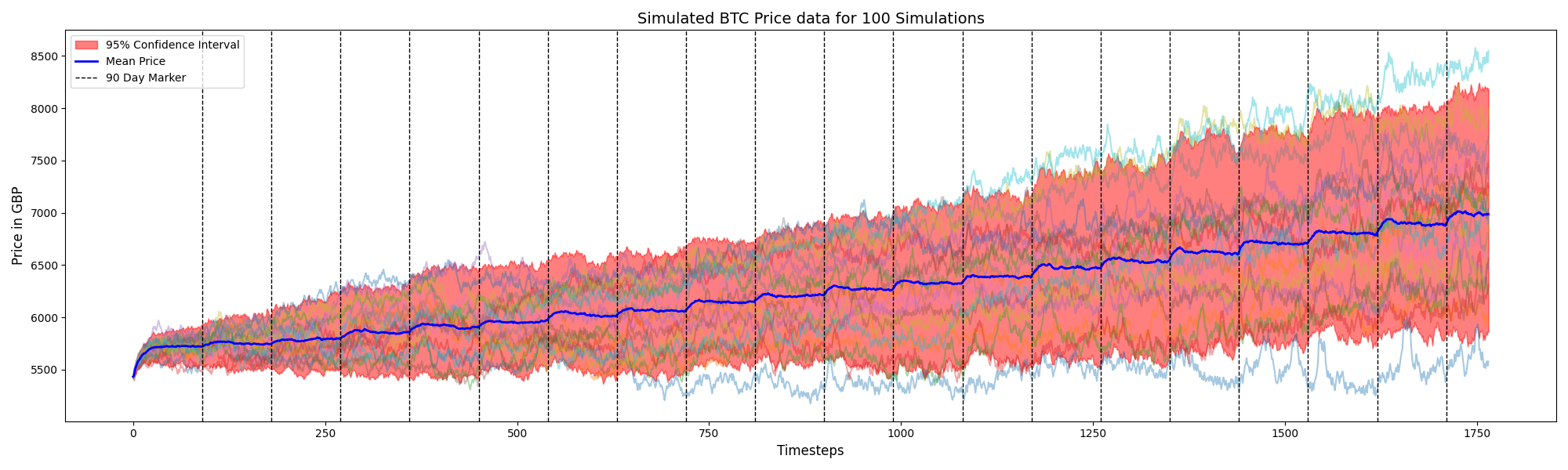
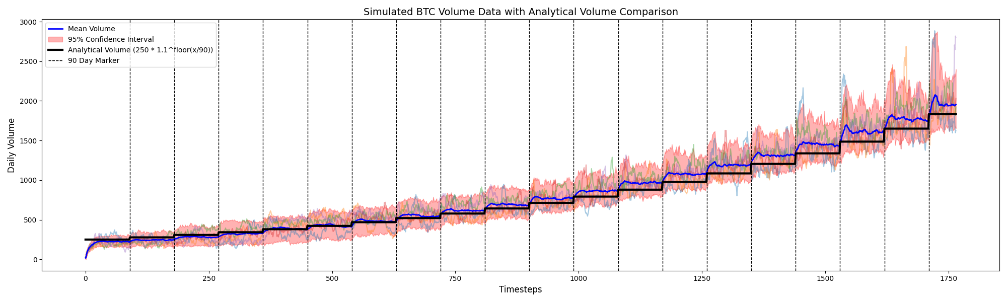
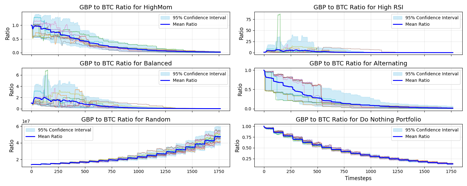
Both frameworks deliver upward-trending prices, but wealth injections induce more realistic surges in this implementation. Volumes also scale closer to observed BTC markets once rescaled by 1,000, because liquidity is not confined to a single cohort of agents.
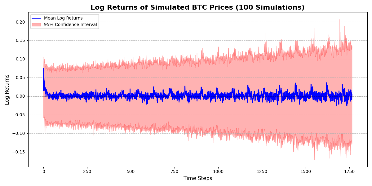
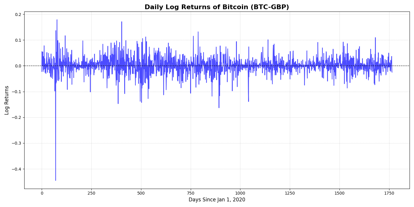
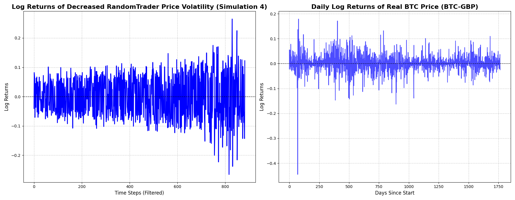
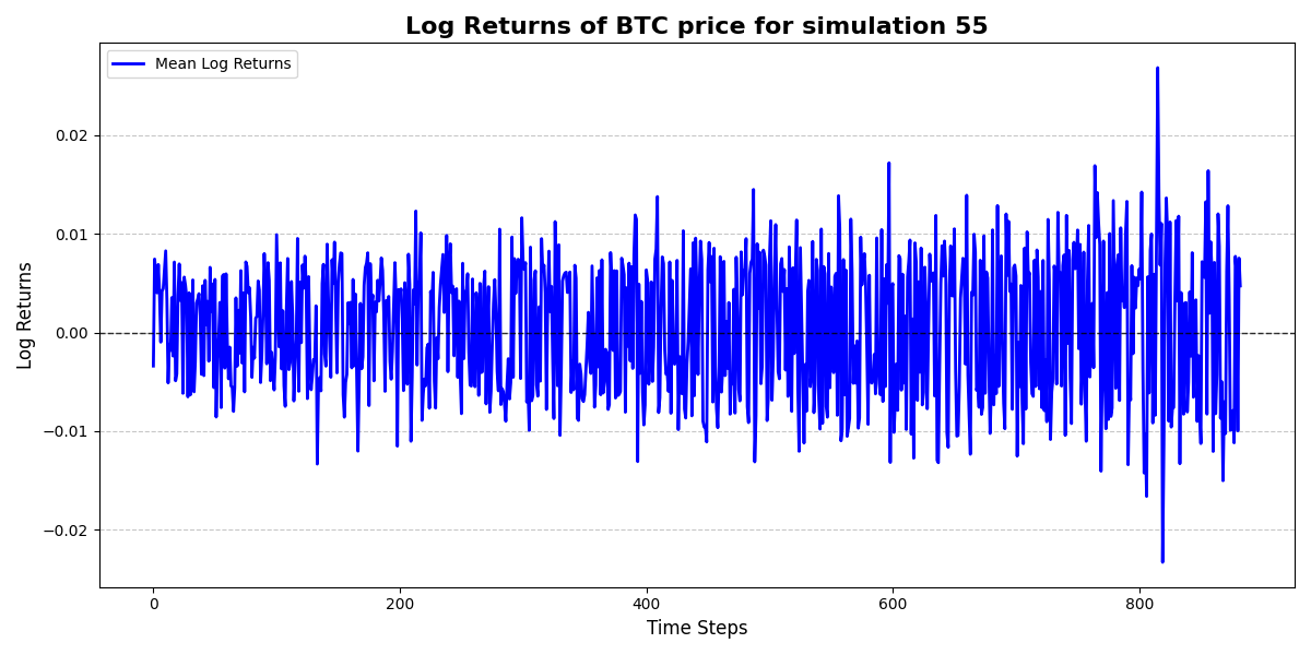
Validation with real BTC data
Log-return distributions match actual BTC-GBP series (2018–2024) and retain volatility spikes between 0.1 and 0.3.

Unit-root behaviour holds under the Augmented Dickey-Fuller test:
| Dataset | Test statistic | p-value |
|---|---|---|
| Real prices | -1.0230 | 0.7448 |
| Log real prices | -1.6028 | 0.4822 |
| Simulated price (mean) | -1.3237 | 0.6213 |
Additional stylised stats:

Takeaways for DBBA Capital
- Momentum plus noise recreates Bitcoin’s signature pathologies. The LOB model delivers fat tails, clustered volatility, and a price process that fails to reject a unit-root null (Cocco et al., 2019).
- Wealth injections act as policy levers. Capital inflows trigger realistic breakouts; withdrawing them returns to a calmer regime.
- Noise traders are essential. They add liquidity, occasionally offset chartist herding, and supply the randomness needed for fat-tailed returns (Dai et al., 2023; Kauffman et al., 2023). Choi et al. highlight how individual traders can distort valuations even in regulated markets (Finance Research Letters).
- Model ready for extensions. Adding transaction costs, fundamentalists, or exchange microstructure quirks would be the next steps to increase realism further (Cocco et al., 2017).