Learning to walk with Novelty Search

NeuroEvolution of Augmenting Topologies

NeuroEvolution of Augmenting Topologies (NEAT) is an evolutionary algorithm for generating intelligent behaviour in one layer neural networks. NEAT works by evaluating neural networks against a fitness function (performance metric) and breeding those networks that perform best. NEAT does not require the backpropogation algorithm or labelled examples to learn, therefore allowing it to be used in much broader settings than deep learning methods. Invented in 2002 by Stanley and Miikkulainen¹ the state of the art adaptations to NEAT have applications in game design², reinforcement learning and control problems³. This article will explore experiments regarding bipedal walking and the NEAT algorithm including its Novelty Search adaptation. Skip to the experiments

The Algorithm

As NEAT is an evolutionary algorithm which obeys the high level process for optimisation shown in the diagram below.

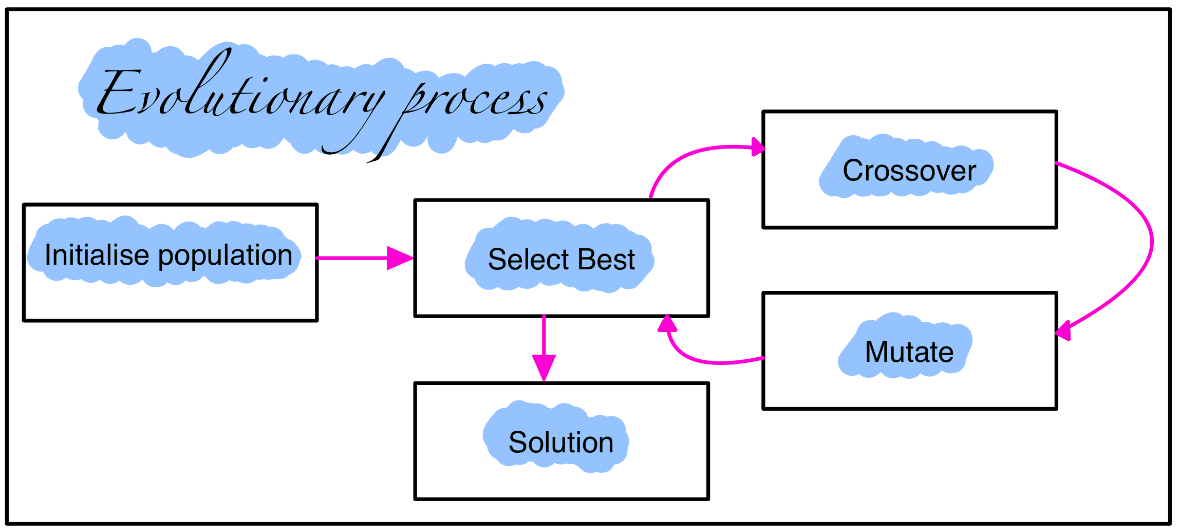
A more detailed description of each step in the evolution process:

1. Initialisation: The first step is to generate a pool of candidate solutions. This can be done by randomly generating neural networks or by loading a set of pre-existing networks.
2. Selection: Next, each candidate solution is assessed on the problem. The best performing solutions are then selected to be parents for the next generation.
3. Crossover: Once the parents have been selected, they are combined to create new solutions. This is done by randomly selecting genes from each parent and combining them to create a new offspring.
4. Mutation: After crossover, the offspring are randomly mutated. This is done by making small changes to the genes of the offspring. Mutation helps to introduce new genetic diversity into the population, which can help to improve the performance of the algorithm.
5. Solution: The NEAT process continues to generate new solutions and assess them on the problem until a solution of sufficient quality is found. Once a satisfactory solution is found, the evolutionary process is stopped and the solution is returned⁴.

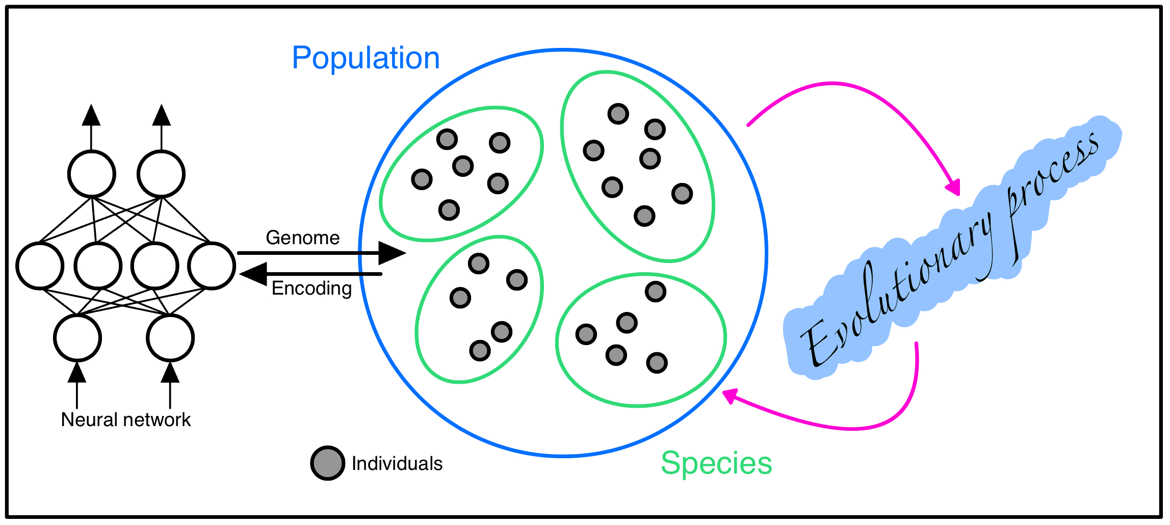
Genetic Encoding

As stated as a key problem in Stanley's paper, a major challenge of NEAT is the genetic representation of the neural networks. It is important to ensure that dissimilar network toplogies can crossover in a meaningful way; new networks are given time to innovate (stopping them being removed from the population prematurely) and finally, how to incorporate Occam's Razor into the problem without a contrived fitness function. These problems are solved in NEAT with the following solutions:

• Utilising historical markings in the genetic encoding to identify topologies with the same origin,
• Separate newly innovated groups into new species,
• Instantiate the network with a minimal structure and only grow when necessary.

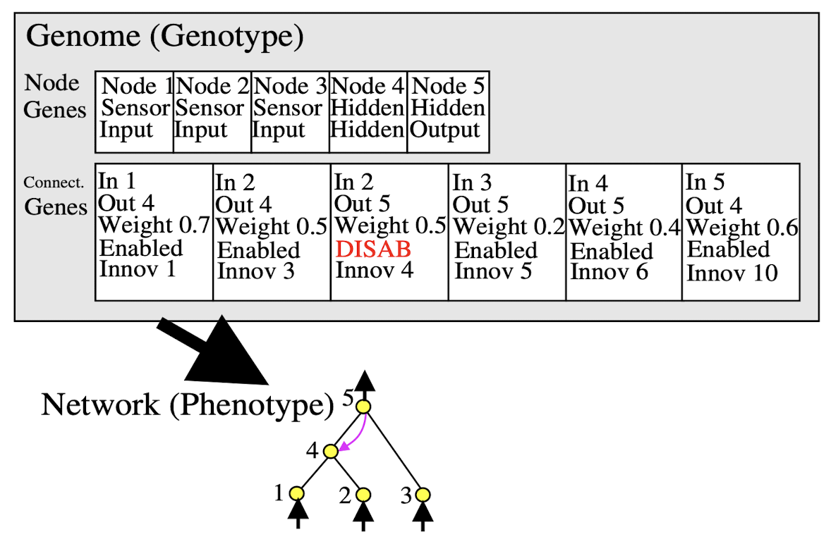
As such, the genetic encoding(genome) for an individual in the NEAT algorithm is as follows:

1. List of node genes defining its activation function and whether it is an input,output or hidden node,
2. List of connection genes where each connection gene specifies the in-node, the out-node, the weight of the connection, an enabled bit and an innovation number (used for crossover).

Mutation

Mutation in NEAT is conducted with the following rules (for each rule it is also possible for nothing to happen to a connection, weight or node):

• Connection weights are perturbed by a random amount,
• A connection is added between two previously unconnected nodes,
• A node is added where a connection was. The old connection is disabled and two new connections are added.

Crossover

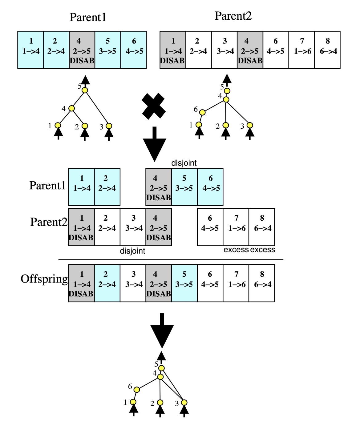
Crossover in NEAT is performed with historical markings, this means whenever a new gene appears (node/connection) a global 'innovation' number is incremented and assigned to that gene. This means that genes with matching innovation numbers can be lined up. Genes that do not match are inherited from the more fit parent or, if they are equally fit, chosen randomly. This method is an incredibly low complexity way to align structure in the parents that is suitable for crossover. An example of crossover is provided below:

Protecting Innovation

Finally, in order to combat the aforementioned problem of the innovations being wiped out before they have time to be optimised we utilise speciation. A distance measure must therefore be created in order to allocated species to individuals in the population. The distance measure ($\delta$) is then defined as a linear combination of excess (E, copies of the same gene) and disjoint(D, genes with not match in the corresponding parent) genes plus the average weight difference of matching genes ($\bar{W}$).

$$\delta = \frac{c_1 E}{N} + \frac{c_2 D}{N} + c_3\bar{W}$$

Where $c_i$ is the importance of each factor and N is the number of genes. A compatibility threshold $\delta_t$ is then defined and each individual is placed into the first species for which its distance is less than the threshold to avoid overlap. Finally, in order to reduce one species dominating the population, NEAT utilises explicit fitness sharing mitigate this. Explicit fitness sharing works by taking every individuals fitness and dividing it by the number of individuals in the species, so we are saying a large species has a better chance to do better and this should be averaged out. Species then grow or shrink depending on their performance relative to the population average.

$$N\_{j}^{'} = \frac{\sum\_{i=1}^{N_j}f\_{ij}}{f}$$

Where:

• $N_{j}$ and $N^{'}_{j}$ are the old updated species size for species $j$,
• $f_{ij}$ is the species size divided individual fitness of individual $i$,
• $f$ is the mean adjusted fitness of the whole population.

Strengths and Weaknesses

NEAT based methods are particularly suited to problems where:

• The problem is dynamic and therefore the neural network needs to be able to fundamentally change throughout its lifetime,
• There is little or no knowledge of the optimal network structure for the problem,
• The gradient of the objective function is degenerate or there are multiple objectives to be simultaneously optimised.

However NEAT performs poorly however in situations where:

• The problem is too expensive to evaluate. NEAT requires evaluating each candidate solution on the problem. If the problem is too expensive to evaluate, then NEAT may not be practical,
• The problem is inexpressible through a one layer neural network, however the adapation to NEAT, HYPER-NEAT⁵ addresses this issue,
• The default encoding scheme in NEAT is not suitable for the network topology that is desired to be developed,
• Limited computational resources because Neuroevolution is incredibly computationally expensive, requiring significant processing power and time, especially for complex tasks.

In particular this article will discuss the fitness and novelty based approaches to NEAT and their accompanying performances on the OPENAI gym bipedal walker environment⁶.

Learning to Walk

The first experiment I attempted was the OPENAI Gym Bipedal Walker environment, the aim was to utilise the NEAT algorithm and learn walking behaviour within a 24 hour training window or by completing the environment (whichever came first). The walker environment is deemed 'completed' if the model can complete 300 units of distance in 1600 time steps and the reward function gives an agent a reward for every unit of distance it travels and penalises an agent for the following:

• The use of any motor joints incurs a small energy cost,
• The walker falling over incurs a -100 score penalty.

Implicitly, this means the environment is telling us a 'good' model is one that travels lots of distance, with minimal energy expenditure and does not fall over. This is a good starting heuristic for 'walking' behaviour, but as will be discussed later, embedding more knowledge into the fitness function improves performance. This leads to my earliest implementation of the function that evaluates a genomes performance as follows:

def eval_genome(genome, config):
    # setup the model and the environment
    env = gym.make("BipedalWalker-v3", hardcore=False,)
    net = neat.nn.FeedForwardNetwork.create(genome,config)
    fitnesses = []

    # run the model in the environment 'runs_per_net' times
    for runs in range(runs_per_net):
        observation, info = env.reset()

        # Run the simulation until environment termination.
        fitness = 0.0
        while True:
            action = net.activate(observation)
            observation, reward, terminated, truncated, info = env.step(action)
            fitness += reward

            if terminated or truncated:
                break

        fitnesses.append(fitness)

    # The genome's fitness is its mean performance across all runs.
    return statistics.mean(fitnesses)

However, after running NEAT in this setup for various hyperparameter settings and a total of 40+ hours of training time, the model would get consistently stuck in a lunging behaviour that gained 6-8 units of distance and then stood still, as demonstrated in the clip below. This behaviour meant that because the walker did not fall over another, more promising, model that travels less than 106 units but falls over is considered worse (once the -100 penalty for falling over is applied) despite have more promising emergent walking behaviour. This problem meant the fitness function is not incentivising walking behaviour well and had to be adapted to avoid this local minima.

Rolling Window Approach

In order to fix the aforementioned problem with the fitness function and a long ignored problem with slow training times I decided to implement a further constraint on the model to address both these issues. These issues were solved by what I called the 'rolling window' approach. This approach gives the model a distance it must attain in a certain amount of time, penalising and ending the simulation run if the model does not attain these criterion. The process is outlined in Figure 5 below.

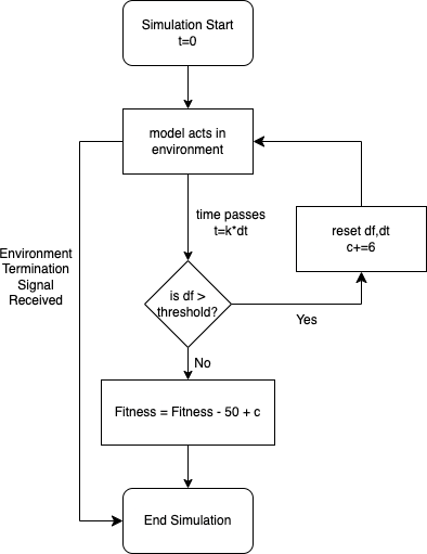
The rolling window approach improves the training process in the following ways:

• The adaptation to the loss function terminates any model that doesnt make it through the next window thereby improving performance (this caused time per generation to go from 20s to 1.2s in my training).
• The adapation penalises any model that doesnt make it through a window(see 'fitness = fitness - 50 + c') thereby incentivising models to move $df$ in $dt$ time and hence alleviating the lunging problem.
• '-50' is selected as the penalty for failing the first window, this is half the penalty for falling over but still sizeable enough to incentivise the walking behaviour desired.
• Finally, in order to ensure that the penalty for failing at window $x$ is less than window $x+1$, $c\\,$ is incremented after every window to make sure the penalty reduces the more windows the model makes it through. After picking 320 and 60 as good candidates for $dt$ and $df$ (when the fifth window is complete the model should have traversed 300 units) the model should complete the environment after making it through five windows.

The code for this approach is as follows:

def eval_genome(genome, config):
    # setup the model and the environment
    env = gym.make("BipedalWalker-v3", hardcore=False,)
    net = neat.nn.FeedForwardNetwork.create(genome,config)
    fitnesses = []

    # run the model in the environment 'runs_per_net' times
    for runs in range(runs_per_net):
        observation, info = env.reset()

        # Run the simulation until environment termination or window failure.
        fitness = 0.0
        time,dt,df,c = 0,0,0,0
        while True:
            time += 1
            dt += 1 % 320

            action = net.activate(observation)
            observation, reward, terminated, truncated, info = env.step(action)
            df = (df + reward)
            fitness += reward

            if terminated or truncated:
                break
            # if the model does not make it through a window
            if dt == 319 and df <= 59:
                fitness =fitness -  50 + c
                df=0
                break
            # if the model makes it through a window
            elif dt == 319 and df > 59:
                c += 6
                df=0

        fitnesses.append(fitness)

    # The genome's fitness is its mean performance across all runs.
    return statistics.mean(fitnesses)

Results

After running the NEAT algorithm with the rolling window setup, convergent walking or 'shuffling' behaviour was achieved after 35000 generations and stagnated until 40000 generations. The training process and final model are displayed in the videos below. Although the model is now moving, albeit inefficiently, the greedy nature of the fitness function means the environment was not completed (the maximum distance attained was 154 units of distance). In order to motivate NEAT to generate more complex walking behaviour, that will not necessarily show dividends straight away, a new fitness function should be considered.

Novelty Search

After listening to the TWiML podcast ⁷ with Kenneth Stanley (the co-author of the original NEAT paper) I discovered novelty search, a supposedly better parameterisation of the fitness function to generate complex behaviour. This new search algorithm is the basis of the second walker experiment. The idea of Novelty Search is to define a fit model as a 'novel' model, this means rewarding solutions that are sparse in the environment space. For example, in a maze (the scenario the paper⁸ uses) a 'novel' solution is one which reaches a new area of the maze rather than minimising something like the distance to the end (which dramatically increases the chance of getting stuck in a local minima).

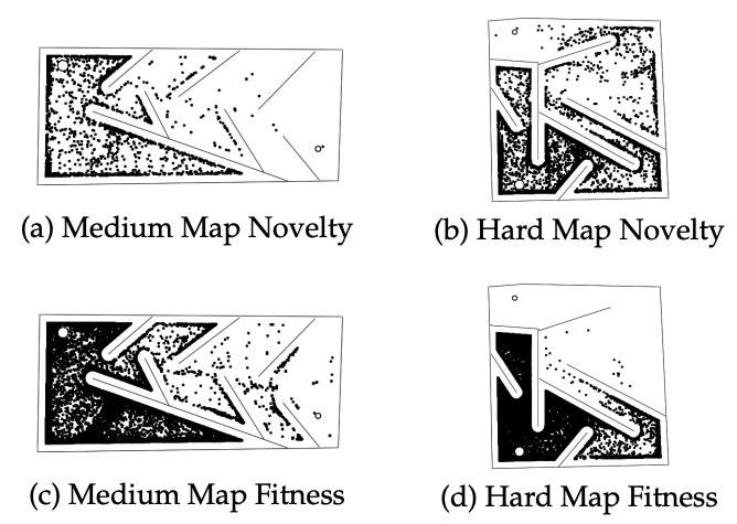
In the example above from Lehman and Stanley's paper on Novelty Search we see that novelty search dramatically outperforms a fitness based approach to maze solving. This setup is applied to the walker environment to see the performance of novelty search. The setup for the algorithm is as follows:

• Novelty is defined as reaching a novel forward distance in the environment i.e the model has walked forwards to a spot no model has reached before,
• A model is not deemed novel if it is within 1 unit of distance to the nearest three models,
• An archive of previous solutions is initially filled with 200 models and then added to whenever a new model is deemed novel,
• The environment is deemed completed if a model completes the 300 units in 1600 time steps.

Therefore, the code for implementing the novelty search is as follows:

def eval_genome(genome, config):
    global archive
    env = gym.make("BipedalWalker-v3", hardcore=False,)
    net = neat.nn.FeedForwardNetwork.create(genome,config)
    fitnesses = []

    for runs in range(runs_per_net):
        novelty = archive.copy()
        observation, info = env.reset()

        fitness = 0.0
        dt,df = 0,0
        while True:
            dt += 1 % 400
            # act on environment
            action = net.activate(observation)
            observation, reward, terminated, truncated, info = env.step(action)
            df = (df + reward)
            fitness += reward
            # early termination heuristic
            if dt == 399 and df < 34:
                df = 0
                terminated = True

            if terminated or truncated:
                if len(archive) < 200:
                    archive.append(fitness)
                    novel = 0
                else:
                    # determine the models novelty
                    novelty = [abs(fitness - x) for x in novelty]
                    novelty.sort()
                    novel = statistics.mean(novelty[:3])
                # if the model is novel add it to the archive
                if novel > 1 and fitness > 0:
                    archive.append(fitness)
                    # if the environment is completed end simultation
                    if fitness >=300:
                        break
                    fitness = novel
                # heuristic to state a non-novel positive model is better
                # than one that falls over
                elif fitness > 0:
                    fitness = -99
                else:
                    fitness = -100
                break

        fitnesses.append(fitness)

    # The genome's fitness is its mean performance across all runs.
    return statistics.mean(fitnesses)

Results

After running NEAT on the new Novelty based fitness function a solution is found to the problem after just 4284 generations (shown in the video below). Although the computational cost is slightly higher than the previous rolling windows approach ($\\approx 5s\\,$ vs $\\approx 1s\\,$), Novelty search took almost 10 times less generations to converge to a solution that travels double the distance of the rolling window approach. Thefore, Novelty Search dramatically outperformed the basic NEAT implementation Below, it can be seen that the final model's behaviour is considerably more complex, utilising more motor joints meaning the algorithm has incentivised learning more complex but meaningful behaviour as desired. Furthermore, in comparison to the distance based approach previously we can see a much more diverse set of optimal architectures being explored by the algorithm.

Conclusion

In conclusion I have learnd a lot about NeuroEvolution in the process of writing this article. In particular, I am glad that my motivation to learn about gradient free learning has led to me discovering these algorithms and I am pleased at the results I have gained. I have learnt about the basic NEAT algorithm and how it can be used in reinforcement learning situations alongside its Novelty Search adaptation. If i was to continue learning more in the area I would look into HYPERNEAT and the more recent developments in the NeuroEvolution space.

Footnotes

1. Kenneth O. Stanley and Risto Miikkulainen , Efficient Evolution of Neural Network Topologies ↩

2. Real-Time Neuroevolution in the NERO Video Game ↩

3. Kenneth O. Stanley and Risto Miikkulainen ,Efficient Reinforcement Learning through Evolving Neural Network Topologies ↩

4. Paul Pauls, A Primer on the Fundamental Concepts of Neuroevolution ↩

5. Kenneth O. Stanley, David D'ambrosio, Jason Gauci A Hypercube-Based Indirect Encoding for Evolving Large-Scale Neural Networks ↩

6. OPEN AI gym Bipedal Walker Environment ↩

7. NeuroEvolution: Evolving Novel Neural Netowrk Architectures with Kenneth Stanley - TWiML Talk 94 ↩

8. Joel Lehman and Kenneth O. Stanley, Abandoning Objectives: Evolution through the Search for Novelty Alone ↩