Creating Maps with Wave Function Collapse

What is Wave Function Collapse/Texture Synthesis?

Skip to Interactive Example

After watching an incredible video by Mark Donald called 'Superpositions, Sudoku, the Wave Function Collapse algorithm'¹, I discovered the Wave Function Collapse Algorithm. In this blog post I will showcase and explain my own implementation of the algorithm and explain the building blocks that allow it to overcome issues affecting the flexibility and generality of the algorithm.

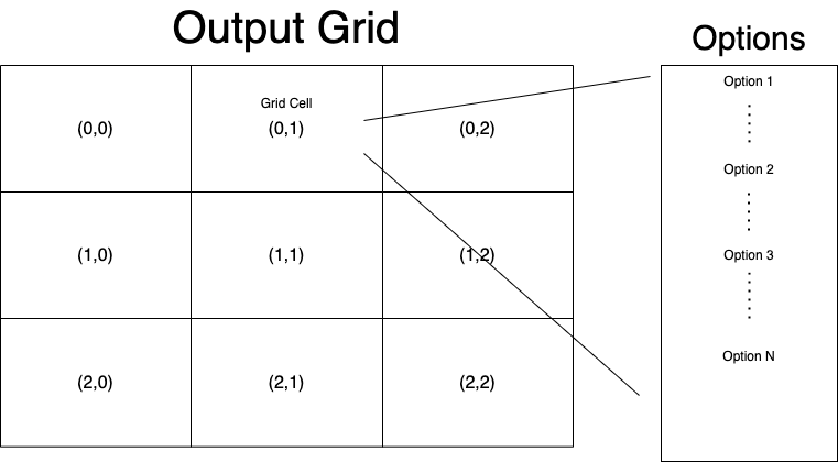
WFC is an algorithm from the larger procedural generation² family that creates content by having a grid of outputs (e.g. pixels, voxels or grid cells) and a set of options, with accompanying probabilities, that could fill each grid cell. The grid cells are then repeatedly filled with the options until a complete image is generated.

The WFC algorithm actually has very little to with quantum physics and is more accurately framed as a constraint satisfaction problem³ solver. Furthermore, it is important to note that Wave Function Collapse (WFC) invented by Gumin⁴ has a sister algorithm Model Synthesis that predates it. WFC generates options from an input image whereas Model Synthesis utilises a predefined set of options.

Implementation

The Algorithm:

In the Algorithm below, items coloured red are implemented in my approach and items coloured in blue will be discussed further later.

• Preliminary: for each option, create a set containing each other option that can be adjacent to that option. We call this set the cell's domain.

1. Select a grid cell to fill,
   • Model Synthesis: Select the cell in scanline order (left->right) then (up->down) OR
   • Wave Function Collapse: Select the cell with the lowest entropy OR
   • Select a random cell,
2. Fix the selected cell's domain:
   • Select an option from the selected cell's domain by sampling from the options probability distribution,
   • Remove all the other options from the cell's domain,
3. For each remaining grid cell in the grid, update their domains based on the newly reduced domain of the selected cell. If there is a cell that has an empty domain:
   • RESET the grid,
   • BACKTRACKING:
     • Return to the last cell to be fixed,
     • Reset its domain to before it was fixed,
     • Remove the tile that was just tried from its domain,
     • Resample from the options probability distribution and fix a new option.

Probabilistic Biome Generation and Shannon Entropy

Throughout the article the idea of 'lowest entropy' has been referred to, in this section the concept will be expanded upon. In particular, at the start of the article it was stated that each option had an accompanying probability. This means, together, the options form a probability distribution with the random variable $\mathbf{x}$ representing a grid cell. Shannon Entropy is a measure of "information" or "uncertainty" in a random variable, and is, for a discrete random variable $\mathbf{X}$ which takes values in $\mathcal{X}$ with probability distribution $p(x)\rightarrow [0,1]$, defined as:

$$H(\mathbf{X})=-\sum_{\mathcal{x}\in \mathcal{X}}p(\mathcal{x})log(p(\mathcal{x}))$$

When Shannon Entropy is "low" (close to zero) there is high certainty about the variable and vice versa. This means Shannon Entropy can be used as the cell selection heuristic because selecting the cell with the fewest options (implying low entropy) decreases the chances of creating a degenerate grid(one where a grid cell has no options in its domain).

Furthermore, custom probability distributions can be crafted (in the case of the City Tileset) for each "Biome" (Grassland, Lagoon, Ocean, Sand or Cave). These "biomes" are subsets of the options organised by some similar attribute, in the case of the CITY tileset this is what type of land the tile is. This allows the user to customise the "maps" that they are creating by weighting biomes differently. This is accomplished by splitting all the options into one of the biomes and calculating its shannon entropy with the probability associated to the biome. So for example by boosting 'Sand' and 'Lagoon' biomes the user is more likely to get a sandy beach or island instead of a grassland area with lots of caves.

Interactive Example

Tilesets:

• Red Grid (Easy) - This is the simplest tileset. There will never be any backtracking as there is an empty tile and an end tile for every direction.
• Red Grid (Hard) - Building on Red Grid Easy, Red Grid Hard takes away the empty tile, end tiles and T junctions to ensure that backtracking will occur for most grids.
• City - The City Tileset is the hardest of the tilesets with 107 tile variations and 5 biomes (Grassland, Desert, Lagoon, Ocean and Walls). It generates video game esque maps up to the 8x8 grid size.

Increasing generality

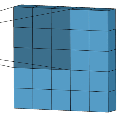
The astute readers may have noticed that, when changing tileset from Red Grid to City, the maximum grid size is reduced from 30 down to 8, this is because the City tileset is considerably more prone to reaching unsolvable states due to the significantly larger set of tiles and inherent incompatibility between tiles from different biomes. In order to remedy this Merrell, in his Ph.D. Thesis⁵, describes an adapation to the WFC algorithm that allows it to drastically increase its chances of solving large grid sizes. The adaptation is called 'Modification in Blocks' and solves the problem by breaking down the grid into smaller subsections then performing the following:

• Precompute: set of known good tiles that will always allow a path to continue beyond the border of a subsection,

1. Select a subsection,
2. Run WFC on the subsection, while adherring to any adjacent subsection's adjacency constraints,
   • When running WFC on the edge of a subsection intersect the domain of the tiles with the set of precomputed "good" tiles,
3. Move the Subsection along so it overlaps the previous subsection by one grid cell.
4. Repeat Until grid is complete.

The subsections are selected in an order that is exactly like a convolutional filter from a Convolutional Neural network and as such Figure 2, adapted from NamyaLG⁶, shows where/how the WFC algorithm is run on the overall grid.

In the future I plan to implement "Modification in Blocks" and to allow the grid size to be increased up to 30 again, a subsequent blog article will follow.

Conclusion

This article explored the Wave Function Collapse (WFC) algorithm, a powerful tool for procedural content generation. It delved into the step-by-step process, from cell selection to resolving conflicts through backtracking. Additionally, the concept of Shannon entropy was introduced, highlighting its value as a metric for guiding cell selection and improving algorithm efficiency.

The limitations of the basic WFC algorithm, particularly with larger or more complex tile sets, were also addressed. The concept of "Modification in Blocks" was presented as a potential solution, with the intention to implement it in a future iteration for generating even more intricate and expansive content. For further exploration, consider checking out Townscaper⁷ by Oskar Stålberg. This game offers a fantastic example of the WFC algorithm in action.

Footnotes

1. Mark Donald, Superpositions, Sudoku, the Wave Function Collapse algorithm ↩

2. Jessica Van Brummelen and Bryan Chen, What is Procedural Generation? ↩

3. Milos Simic, Michal Aibin Constraint Satisfaction Problems ↩

4. Maxim Gumin, Wave Function Collapse ↩

5. Paul Merrell, Model Synthesis ↩

6. NamyaLG, What is 2-Dimensional Convolution? ↩

7. Oskar Stålberg, Townscaper ↩