The Spatial Ecology of Predator-Prey Systems.

Abstract

This study focuses on two methods of computationally modelling systems of many interacting particles of two species. The first method is the general idea of reaction-diffusion systems, which are mathematical differential constructs that describe how spatial and temporal patterns can emerge from the interactions between mathematical species and their environment. Also considered are agent based models, which instead only use hyper-local information and do not rely on macroscopic differential equations at all. In particular, the predator prey system is considered from both perspectives. By coupling local interaction rules with movement, these models elucidate the dynamics of population spread, predator-prey relationships, and the emergence of patterns in ecosystems.

Introduction to reaction-diffusion systems

Theoretical ecology is a mathematical framework for understanding how the interactions of individual organisms with each other and with the environment determine the distribution of populations and the structure of communities. Many different models are needed, each based on some set of hypotheses about the scale and structure of the spatial environment and the way that organisms disperse through it. When many agents interact in simple ways, sometimes emergent properties can be observed in their collective, such as the propagation of wavefronts or the formation of patterns. These patterns are glimpses of structure from chaos, and have prompted countless minds to become fascinated by the connections between maths and biology.

Reaction-diffusion models are a way of translating the simple assumptions about ways agents can move and interact on the local level into global conclusions about the persistence or extinction of populations and the coexistence of interacting species. Born from the macroscopic observations of molecular diffusion, reaction-diffusion models now more widely refer to any event-driven system of interacting moving agents, and occur and many different scales.

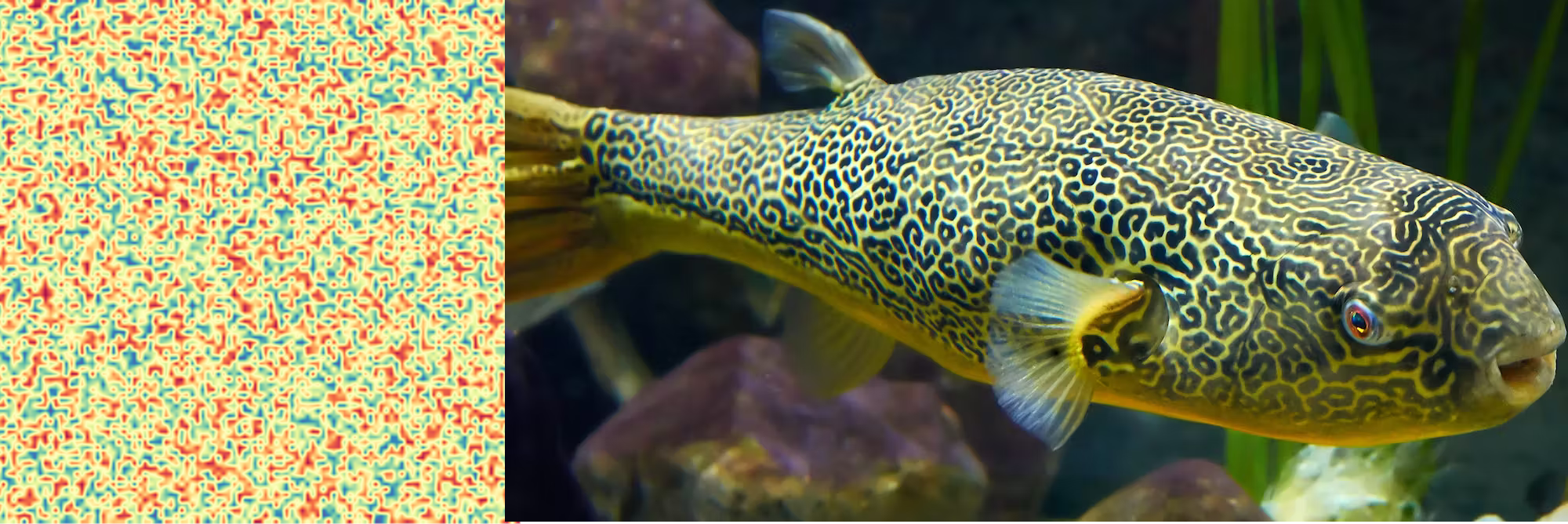
In biology, the great success of reaction-diffusion mathematics is the Turing model, which describes how homogeneous groups of cells in an embryo can spontaneously differentiate into patterns, like the spots and stripes on animal skins [1]. In chemistry, the Belousov-Zhabotinsky chemical reaction is an incredible display of dispersive concentric patterns. Further examples are as distributed as econometric information diffusion and as grievous as modelling the spread of forest fires.

These systems are linked, and the outcomes we see from their patterns are directly caused by similarities in the form of the differential equations which govern their spatio-temporal evolution. They share the two species reaction diffusion equations, which are given by

$$\begin{equation} \begin{pmatrix} \dot q_{1} \\\ \dot q_{2} \end{pmatrix} = \begin{pmatrix} D_{1} \\\ D_{2} \end{pmatrix} \cdot \nabla^{2} \begin{pmatrix}q_{1} \\\ q_{2} \end{pmatrix} + \begin{pmatrix} R_{1}(q_{1}, q_{2}) \\\ R_{2}(q_{1}, q_{2}) \end{pmatrix}, \end{equation}$$

where $q_{1,2}$ describes the concentration of either species, $D_{1,2}$ their diffusion coefficients, and $R_{1,2}(q_{1}, q_{2})$ are functions representing the agent's interactive and local behaviour. Decomposing the equation, the first term on the right hand side can be recognised as Fick’s second law of diffusion, $\dot q = D \nabla^{2} q$ for a concentration $q$ [2].

The dynamics of our model is specified by the rates at which individuals move and die or reproduce. As such, a good place to start is to consider the local mechanics of our agent movement and reactions, supposing that agents may only move to a randomly chosen nearest neighbour of their location, and reproduce or die at rates which depend on the number of individuals at the same location. Using some simplifying assumptions along the way, there are creative ways to derive the reaction term, which is usually, hopefully, linear in $q_{1,2}$. Often, however, we are not so lucky. Spatial models often unavoidably invite non-linear terms, resulting in chaotic long-term behaviour.

Agent based models for two species populations

Spatial ecology can also be modelled computationally using agent-based models, and the benefit of this is that it did not assume the truth of a set of universal differential equations. As such, agent based models offer a completely different method for simulating systems of interacting particles by operating exclusively at the local level, with no macroscopic information shared to individual agents. Diffusion occurs via steps in random directions. Reactions occur based on only local information, such as if two interacting agents of the same species at the same place have enough energy to procreate. While these models are much closer approximations to real life, they still lack the macroscopic dynamics of flocking, herding, fleeing, or hunting. As such, it may make sense to imagine these agents as small groups of microorganisms, diffusing due to the random flow of Brownian motion, rather than intelligent autonomous animals.

Design considerations

Energy

Prey generate energy stochastically but passively, and will do so as long as they are not eaten. Predators can only generate energy by feeding on prey. Energy on average is gained rather than lost throughout the simulation. However, existing in the same gridsquare as another agent of your own species incurs an energy cost directly proportional to the number of agents there. For example, if $40$ agents occupy the same gridspace, they will each suffer an energy cost of $40$ energy that iteration. This is meant to replicate an energy cost due to limited food supply at any one area, and makes the populations display self-limiting behaviour.

Procreation

To procreate, agents must bump into each other on the same gridspace, and if both parents have above a minium energetic threshold, they will procreate and suffer an energy cost. There is no limitation on procreating with your own offspring. To avoid extinction in my simulations, parthogenetic (asexual) procreation is made possible when species populations dwindle too low.

What can the agent based model tell us?

Emergent properties from the simulation can be seen, such as expanding wavefronts of prey being chased down by a wavefront of predators, feasting on the stragglers.

Explosive pockets of mass generations of new agents can be seen, but why do they occur? The spatial and energetic restrictions on when procreation can occur sometimes impede local procreation rates, which can lead to huge gains in agent energy. As enough energy gets stored up and the species begins to bump into itself, a chain reaction of procreation is set-off. The limiting factor of this is usually the rate of diffusion, which leads to most agents in the chain reaction dying due to the energy cost of occupying the same gridsquare as many others before they can move away to safer areas.

Lotka-Volterra equations

Without spatial dependence

The Lotka-Volterra equations, are a mathematical model for the population dynamics of a predator species and a prey species, perhaps foxes and rabbits, and is a convinient way to explore how reaction terms work. Choosing to completely ignore spatial dimensions, the mean field assumption can be adopted: that all agents interact with the average effect of all others. Letting $x_1(t)$ denote the prey population and $x_2(t)$ denote the predator population at time $t$,

$$\begin{equation} \dot x_1 = \alpha x_1 - \beta x_1 x_2, \dot x_2 = \delta x_1 x_2 - \gamma x_2. \end{equation}$$

• $\alpha$ is the natural birth rate of the prey in the absence of predators.

• $\beta$ is the death rate of the prey due to predation.

• $\gamma$ is the natural death rate of the predators in the absence of prey.

• $\delta$ is the rate at which predators increase by consuming prey.

Reading off from the general form of reaction-diffusion equations, $D_1$ and $D_2$ have been set to zero, and the remaining terms are the reactive terms $R_{1,2}(q_{1}, q_{2})$. Below, linear stability analysis is used with the method outlined by Strogatz [3] pp.151-152]. Firstly, the steady states of this system of differential equations are found by setting the time derivatives to zero. The trivial solution $x_1 = x_2 = 0$ indicates mutual extinction, but otherwise, solving for constants, we get

$$\begin{equation} x_1, x_2 = \gamma / \delta, \alpha / \beta. \end{equation}$$

Secondarily, to analyse the stability of these steady state solutions, our set of differential equations are linearised so that we have

$$\begin{equation} J = \begin{pmatrix} \frac{\partial f_1}{\partial x_1} & \frac{\partial f_1}{\partial x_2} \\\ \frac{\partial f_2}{\partial x_1} & \frac{\partial f_2}{\partial x_2} \end{pmatrix} = \begin{pmatrix} \alpha - \beta x_2 & -\beta x_1 \\\ \delta x_2 & \delta x_1 - \gamma \end{pmatrix} = \begin{pmatrix} 0 & -\beta \frac{\gamma}{\delta} \\\ \delta \frac{\alpha}{\beta} & 0 \end{pmatrix}. \end{equation}$$

The trivial solution has eigenvalues $\alpha$ and $-\gamma$, indicating a saddle point 3, p.130]. This is good, because saddle points are unstable, meaning the model does not predict spiralling uncontrollably towards extinction. The other matrix has eigenvalues $+i \sqrt{\alpha \gamma}$ and $- i \sqrt{\alpha \gamma}$, which indicates periodic trigonometric-esque solutions. We can see this in the graph, that for the original Lotka-Volterra equations no matter how close either species gets to zero, they always bring it back from the brink.

The model elegantly captures the core ideas: prey populations grow naturally but are eaten by predators, and predator populations decline without food but grow when they eat prey. That said, the model is limited, as it never predicts extinction for nonzero initial populations. A better model would include a notion of self competition in the individual populations, perhaps stemming from a fixed supply of food. Such a model would be self-limiting. A better model,

$$\begin{equation} \dot x_1 = \alpha x_1 (1 - x_1 / \eta_{1}) - \beta x_1 x_2, \dot x_2 = - \gamma x_2 + \delta x_1 x_2 \end{equation}$$

introduces the notion of independent growth limitation on the individual populations $x_1$ and $x_2$ to the system through the Logistic model. The terms $\eta_1$ and $\eta_2$ represent the carrying capacities, a concept from ecology that refers to the maximum population size of a species that the environment can sustain indefinitely, given the food, habitat, water, and other necessities available in the environment. In mathematical models like this one, the carrying capacity limits the growth of a population by introducing a term that reduces the growth rate as the population size approaches the carrying capacity. The advantages is this allows one species to “win”, in addition to cases where both populations settle on fixed values.

Adding spatial dependence

The main ingredient missing from these models is the absence of spatial dependence in the model. There is reason to be concerned with the mean field assumption that we adopted before, which states that all agents interact with the average effect of all the others agents, irrespective of their physical distance from them. In the next step of this model, the agents will exist in 2D space, and will only interact with their immediate spatial neighbours.

One option is to add in our our Fick’s law inspired diffusion terms, and so we define the spatial Lotka-Volterra equations

$$\begin{equation} \frac{\partial x_1}{\partial t} = \alpha x_1 - \beta x_1 x_2 + D_1 \nabla^2 x_1, \end{equation}$$ $$\frac{\partial x_2}{\partial t} = \delta x_1 x_2 - \gamma x_2 + D_2 \nabla^2 x_2.$$

We have found our set of reaction-diffusion equations for the predator-prey model, with the reaction part handled by the Lotka-Volterra.

Reaction-diffusion simulation using RK4

This set of differential equations can be modelled computationally on a randomised initial population to show the progression of the non-linear system. The Runge-Kutta (RK4) method is used for executing this progression by a timestep $dt$. As before, the colour green represents prey, and the colour red represents predators.

You may have to click through some blanker periods, but a gif of the progression is given at the bottom of the page.

Some interesting patterns can be seen to form. There seems to be at times stripes and dots with a characteristic length, and we recall the Turing patterns mentioned before. Are these Turing patterns that we are seeing?

Another unignorable characteristic is the end result of the horizontal stripes. This may be a fragment of the simulation when discretised into a grid, or a quirk of the RK4 method, or a by-product of the simplified Laplacian in the setting of the 2D grid.

Turing patterns in the spatial Lotka-Volterra equations

When do Turing patterns occur?

Turing patterns occur due to a mathematical feature of the system's governing differential equations. 'Turing instability' is a measure of the tendency of a homogeneous state in such systems to become unstable and spontaneously give rise to spatial patterns.

For Turing instability, we need [6]:

• the homogeneous system to be stable without diffusion, which we proved in the linear stability analysis in the previous section,
• and the diffusion terms to destabilize the homogeneous steady state.

This second condition is possible to prove by linearising the differential equation system, and finding its eigenvalues. Assuming $u$ and $v$ have solutions of the form $e^{\lambda t + ik\cdot r}$, we can solve the characteristic equation to get a disperstion relation between $\lambda$ and $k^2$. We will have achieved condition 2 and proved the existence of diffusion-driven instability if we can show that the real part of $\lambda$ is at any point positive for some range of $k^2$.

Are we seeing Turing patterns?

Let's remind ourselves of our reaction-diffusion system.

$$\begin{equation} \frac{\partial x_1}{\partial t} = \alpha x_1 - \beta x_1 x_2 + D_1 \nabla^2 x_1 \end{equation}$$ $$\frac{\partial x_2}{\partial t} = \delta x_1 x_2 - \gamma x_2 + D_2 \nabla^2 x_2$$

To prove that the given system of equations produces Turing patterns [4], we need to perform a linear stability analysis around a homogeneous steady state solution, and look for conditions under which perturbations grow in a spatially inhomogeneous way. We will follow the method here [5]. First, let's find the homogeneous steady state $(x_1^{*}, x_2^{*})$ for a spatially uniform state by setting

$$\begin{equation} \frac{\partial x_1}{\partial t} = \frac{\partial x_2}{\partial t} = 0, \nabla^2 x_1 = \nabla^2 x_2 = 0. \end{equation}$$

Subbing this into the above spatial Lotka Volterras, we get

$$\begin{equation} 0 = \alpha x_1^* - \beta x_1^* x_2^*, 0 = \delta x_1^* x_2^* - \gamma x_2^*. \end{equation}$$

Solving for $x_1^{*}$ and $x_2^{*}$,

$$\begin{equation} x_2^{*} = \frac{\alpha}{\beta} \end{equation}$$

and

$$\begin{equation} x_1^* = \frac{\gamma}{\delta x_2^{*}} = \frac{\gamma \beta}{\alpha \delta} \end{equation}$$

Next, we linearize the system around the steady state by letting $x_1 = x_1^* + u$ and $x_2 = x_2^* + v$, where $u$ and $v$ are small perturbations. We then substitute these into our system and keep only linear terms in $u$ and $v$. After linearization, the system becomes:

$$\begin{equation} \partial_t u = \alpha u - \beta (x_1^* v + x_2^* u) + D_1 \nabla^2 u \end{equation}$$ $$\partial_t v = \delta (x_1^* v + x_2^* u) - \gamma v + D_2 \nabla^2 v$$

Substituting the steady-state values and simplifying we get

$$\begin{equation} \partial_t u = (\alpha - \beta x_2^*) u - \beta x_1^* v + D_1 \nabla^2 uu = - \frac{\beta \gamma}{\delta} v + D_1 \nabla^2 u \end{equation}$$ $$\partial_t v = \delta x_2^* u + (\delta x_1^* - \gamma) v + D_2 \nabla^2 v = \delta x_2^* u + (\delta x_1^* - \gamma) v + D_2 \nabla^2.$$

So, we have our fully linearized system which we can write in matrix form as:

$$\begin{equation} \begin{pmatrix} \partial_t u, \\\ \partial_t v \end{pmatrix} =\begin{pmatrix} D_1 \nabla^2 & -\frac{\beta \gamma}{\delta} \\\ \frac{\alpha \delta}{\beta} & D_2 \nabla^2 - \gamma \end{pmatrix} \begin{pmatrix} u \\\ v \end{pmatrix} \end{equation}$$

Now we look for solutions in the form of $e^{\lambda t + ik\cdot r}$, where $\lambda$ is the growth rate of the perturbation, $k$ is the wave number, and $r$ is the position vector.

We substitute this form into the linearized system and solve for $\lambda$. Given the reaction-diffusion system is now linearised, we can now find the eiganvalues, $\lambda$, and this ends up giving us a dispertion relation for the perturbation:

$$\begin{equation} \det \begin{pmatrix} D_1 k^2 - \lambda & -\frac{\beta \gamma}{\delta} \\\ \frac{\alpha \delta}{\beta} & D_2 k^2 - \gamma - \lambda \end{pmatrix} = 0 \end{equation}$$

Solving the characteristic equation, we get:

$$\begin{equation} (D_1 k^2 - \lambda)(D_2 k^2 - \gamma - \lambda) - \left(-\frac{\beta \gamma}{\delta}\right)\left(\frac{\alpha \delta}{\beta}\right) = 0 \end{equation}$$

Expanding and simplifying gives us a quadratic equation in $\lambda$,

$$\begin{equation} \lambda^2 + \lambda(D_1 k^2 + D_2 k^2 - \gamma) + h(k^2) = 0. \end{equation}$$

where $h(k^2) = D_1 D_2 k^4 - \gamma D_1 k^2 - \alpha \gamma$.

As outlined here, if we look for a sign change in the real part of $\lambda (k^2)$, this indicate there exists a range of wavenumbers for which patterns will emerge. The range for which it is positive will give us the characteristic length of the Turing pattern.

Instead, we will reason that if we have $h(k^2) < 0$ for some $k^2$, it must be true that $\lambda(k^2)$ is positive for that same interval of $k^2$, because of the positive $\lambda$ coefficients in $\lambda^2 - \lambda(D_1 k^2 + D_2 k^2 - \gamma) + h(k^2) = 0.$

Next, performing a quick change of variables $z = k^2$,

$$\begin{equation} \frac{dh(z=k^2)}{dz}=2 D_1 D_2 z - \gamma D_1, \end{equation}$$

we aim to find the stationary point so set $\frac{h(z^{*})}{dz}$ to zero, and prove its minimum is negative. We get $z^{*}=\frac{\gamma}{2 D_2}$, and plugging this into $h(z)$ gives a value for $h_{min}$ (since $h(z)$ is clearly concave),

$$\begin{equation} h_{min}(z^{*}=\frac{\gamma}{2 D_2}) = \frac{D_1 D_2 \gamma^2}{4 D_2} - \frac{D_1 \gamma^2}{2 D_2} - \alpha \gamma = - \frac{D_1 \gamma^2}{D_2} - \alpha \gamma \end{equation}$$

Since $\alpha, \gamma, D_1, D_2$ are necessarily $>0$, we have proved that for $h(k^2)$ is necessarily negative for some range of $k^2$, and that $\lambda$ is positive for that same range of $k^2$.

By solving for the roots of equation (17), we find that $k^2$ is positive for the range:

$$\begin{equation} \frac{D_1 \gamma - \sqrt{D_1 \gamma (D_1 \gamma + 4 D_2 \alpha)}}{2 D_1 D_2} < k^2 < \frac{D_1 \gamma + \sqrt{D_1 \gamma (D_1 \gamma + 4 D_2 \alpha)}}{2 D_1 D_2}. \end{equation}$$

The characteristic length of the Turing patterns in our system is therefore:

$$\begin{equation} L_c = \frac{\sqrt{D_1 \gamma (D_1 \gamma + 4 D_2 \alpha)}}{D_1 D_2}. \end{equation}$$

Conclusion

Feel free to check out my github..

The agent based model was the most enjoyable, the most challenging, and took the most time. For performance reasons, the backend had to be rewritten in C#, and is now hosted on Azure so it can be run on demand. The graphing occurs via saving the image to a binary array and then displaying it simply as a base-64 encoded string. This model could easily be used for further research or study. For instance, agent based models have recently become hugely important in predicting the mature structure of bacterial biofilms, particularly to mirror how biofilms react to stimuli in lab scenarios.

Modelling the reaction diffusion equations in the browser was an interesting challenge. As promised, here is the .gif of the progression of the simulation.

References

1. Turing, A. “The Chemical Basis of Morphogenesis.” Bulletin of Mathematical Biology, vol. 52, no. 1–2, Jan. 1990, pp. 153–97.

2. Wikipedia Contributors. “Fick’s Laws of Diffusion.” Wikipedia, Wikimedia Foundation, 14 Nov. 2023, en.wikipedia.org/wiki/Fick%27s_laws_of_diffusion#Fick. Accessed 18 Nov. 2023.

3. Strogatz, Steven, author. Nonlinear Dynamics and Chaos : with Applications to Physics, Biology, Chemistry, and Engineering. Boulder, CO :Westview Press, a member of the Perseus Books Group, 2015.

4. Bois, J and Elowitz, M (2019) 'Turing patterns' CalTech

5. Perthame, B. 2015. Linear Instability, Turing Instability and Pattern Formation. Lecture Notes on Mathematical Modelling in the Life Sciences, pp. 117–143.

6. Haas, P.A. and Goldstein, R.E., 2021. Turing’s diffusive threshold in random reaction-diffusion systems. Physical Review Letters, 126(23), p.238101.